Steepest Descent (SD)

Overview

The steepest descent optimizer moves each step directly along the negative gradient direction, scaled by a fixed maximum step length. It is the simplest first-order method and requires no history or Hessian information. Invoked with method=sd inside #opt().

Because each step is independent and the direction is always the steepest downhill direction, SD is highly robust for severely distorted geometries but converges slowly near a minimum due to its tendency to zigzag. For better convergence after the initial descent, consider switching to CG or using the automatic SD/CG fusion.

Parameters

Parameter	Type	Default	Description
`max_step`	float	`0.2`	Maximum step length in Angstrom.
`max_iter`	int	`256`	Maximum number of optimization cycles.
`sd_max_iter`	int	`50`	Maximum SD iterations before stopping (when used as a standalone method).
`write_traj`	bool	`False`	Write intermediate geometries to a trajectory file.
`traj_every`	int	`1`	Write trajectory frame every N steps.
`verbose`	int	`1`	Output verbosity level.

Input Example

#model=uma
#opt(method=sd)
#device=gpu0

C      -0.77812600     -1.06756100      0.32105900
C       1.30255300      0.05212000     -0.02829900
C      -0.97199300      1.45624900      0.82365700
C       1.98122900     -0.41843300      1.25017500
C       2.26403300      0.43516800     -1.13310700
N       0.29116400     -0.87682100     -0.50039900
N      -2.01916300     -1.37200600     -0.23311200
O      -1.66473400      1.63022300     -0.40183700
H      -2.25863200      0.87013900     -0.47589900
H       0.02784900     -0.67831200     -1.45849500
H      -0.60975900     -1.36785600      1.34117800
H       0.68126400      0.91830000      0.28694100
H      -2.57326300     -2.05736100      0.25741200
H      -2.05242800     -1.50454200     -1.23382300
H      -0.36899300      2.35139200      0.99174700
H      -1.63960900      1.29421500      1.67465300
H       2.76444900      0.29146200      1.52284600
H       1.72511400      0.73069500     -2.03779400
H       2.43559300     -1.40609800      1.13421500
H       1.27300500     -0.44722400      2.08057900
H       2.85034500      1.29869700     -0.81432200
H       2.96000900     -0.36880600     -1.38891000

When to Use

Severely distorted geometries: When the starting structure has large steric clashes or unreasonable bond lengths, SD rapidly reduces the worst forces without requiring Hessian information.
Pre-optimization pass: A short SD run can stabilise a structure before handing off to a more efficient method such as L-BFGS or RFO.
Diagnostic runs: Because each step is independent and the algorithm is transparent, SD is useful for isolating convergence problems.

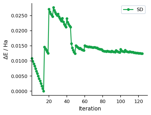
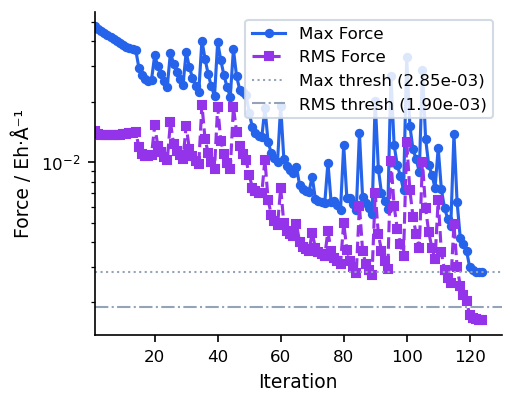
Convergence Behaviour

The figures below show a typical SD run on a 22-atom organic molecule (UMA model). Energy drops steeply in the early iterations but the characteristic zigzagging of SD slows convergence near the minimum.

SD energy vs iteration — Fig. 1 — Energy convergence (SD)

SD force vs iteration — Fig. 2 — Force convergence (SD)

Note

Pure SD is rarely the best choice for a complete optimization. Consider SD/CG to automatically transition to conjugate gradient once the large initial forces have been reduced, or L-BFGS for production runs.