IRC: Euler Predictor–Corrector (EulerPC)

Overview

EulerPC (Euler predictor-corrector) is a first-order predictor-corrector IRC integrator designed to achieve a favorable trade-off between computational cost and accuracy. Due to the first-order nature of the predictor step, EulerPC often requires smaller step sizes or a higher density of path points to reach a level of precision comparable to higher-order or Hessian-based methods (such as GS or HPC), which may lead to reduced efficiency in certain cases. However, it serves as a robust and practical alternative when Hessian-based methods are unavailable, computationally prohibitive, or numerically ill-behaved.

Like HPC, it uses the Modified Bulirsch-Stoer integrator on a DWI surface to refine the path.

Algorithm

At each IRC step, the EulerPC method proceeds in three phases:

Predictor — Following an initial displacement along the transition vector corresponding to the imaginary frequency, an Euler predictor step is performed in mass-weighted coordinates.
Evaluation — The potential energy surface derivatives are evaluated at the predicted point, and a locally fitted PES is constructed using information from both the starting and predicted points.
Corrector — A correction integration is performed on this local surface to mitigate path deviations resulting from finite step sizes.

Parameters

The complete EulerPCParams dataclass:

Parameter	Type	Default	Description
`target_mode`	int	1	Index of the imaginary mode to follow.
`step_length_bohr`	float	0.10	Step length in Bohr.
`max_steps`	int	50	Maximum IRC steps per direction.
`max_pred_steps`	int	500	Maximum predictor sub-steps.
`loose_cycles`	int	3	Number of initial cycles with loosened convergence.
`hessian_recalc`	int	None	Recalculate Hessian every N steps.
`hessian_update`	str	`bofill`	Hessian update: `"bfgs"` or `"bofill"`.
`dwi_n`	int	4	Distance-weighted interpolation points.
`mbs_max_k`	int	15	Max polynomial order for MBS.
`mbs_points`	int	20	Number of MBS integration points.
`mbs_tol`	float	1e-5	MBS convergence tolerance.
`f_max_th`	float	2e-3	Max force convergence threshold.
`f_rms_th`	float	5e-4	RMS force convergence threshold.
`print_each`	bool	True	Print details at each IRC point.
`write_traj`	bool	True	Write trajectory XYZ files.

Example: Radical isomerization

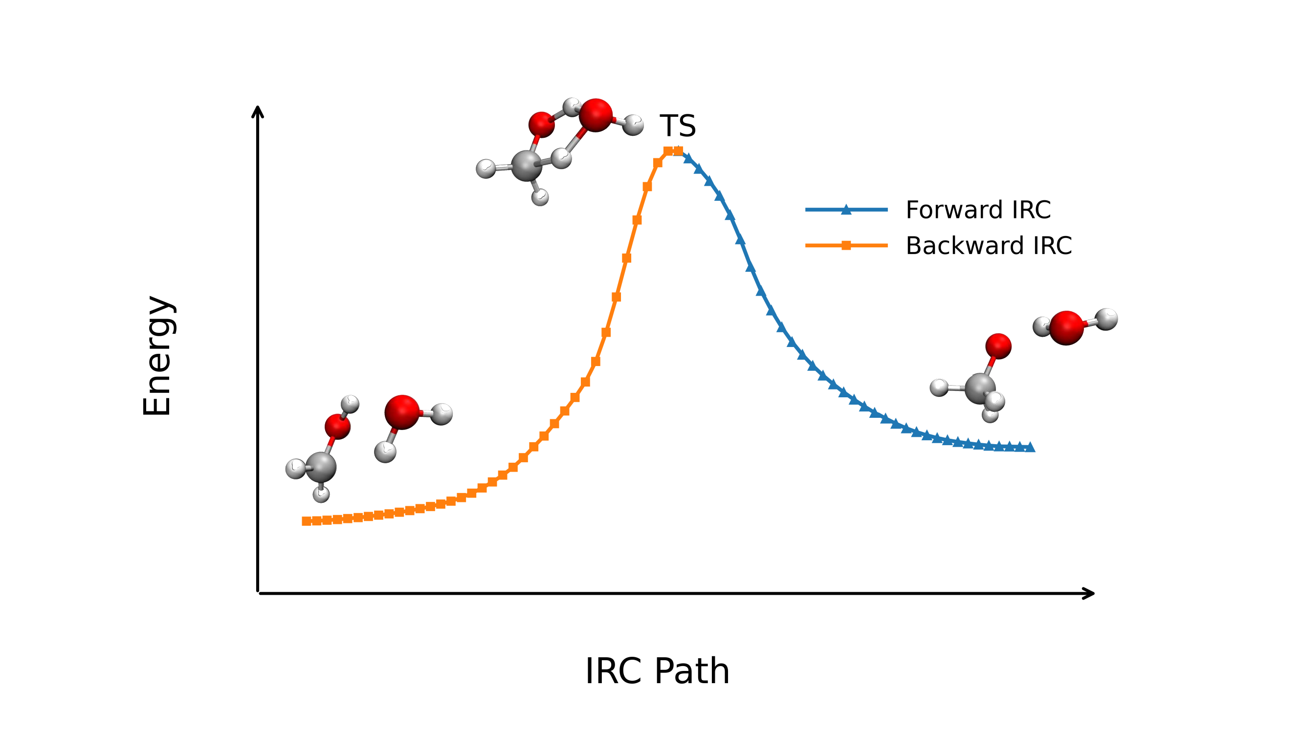
In this example, we will perform the calculations for the H2COH -> H3CO reaction involved in the original EulerPC reference. The TS structure is derived via the String method and the explicit water is considered to assist the reaction, with the system having a spin multiplicity of 2.

Input Example

#model=aimnet2nse
#irc(method=eulerpc)
#device=gpu0

XYZ  0  2  /path/to/transition_state.xyz

Output Visualization

After a brief wait for the calculation to complete, we can visualize the reaction path and the energy profile along the reaction coordinate.

EulerPC IRC animation — **Trajectory:** Simplified view of the reaction path

EulerPC IRC graph — **Graph:** Energy trend along the IRC path

Ref Structure

Transition State

8
Image 0  Energy = -191.55241663
C   0.2707493323 -0.8839208040  0.0593391556
H   0.8065677208 -2.2033699236  0.4439009220
H   0.8020890579 -0.6010813154 -0.8576257232
H  -0.8079751217 -1.0413748042 -0.0556802194
O   0.7091869188 -0.3944101545  1.2167602799
O   1.3829694247 -2.5998174092  1.4932190528
H   2.3408200175 -2.6386038898  1.3632820341
H   1.1873343825 -1.4974192399  1.7123875960

Comparison of IRC Methods

Method	Speed	Robustness	Best For
GS	Moderate	High	General use and path curvature sensitive
LQA	Fast	Moderate	Smooth surfaces
HPC	Moderate	High	Balanced speed/accuracy
EulerPC	Fast	Moderate	Wish to use Euler's integral

When to Use

The EulerPC method is recommended as a fallback when other IRC methods have difficulty:

When the default HPC method, LQA, or GS fail to converge along the IRC path.
For reactions involving large-amplitude motions or irregular PES regions.

For routine IRC calculations on well-behaved surfaces, the GS method or the default HPC method are generally preferred.