IRC: Local Quadratic Approximation (LQA)

Overview

The Local Quadratic Approximation (LQA) method is an IRC integration algorithm that approximates the potential energy surface locally by a second-order expansion in mass-weighted coordinates. the LQA method solves the differential equation of motion analytically on this quadratic surface using the eigenvalues and eigenvectors of the mass-weighted Hessian. This allows the path to "curve" correctly within a single step. On smooth, well-behaved potential energy surfaces, LQA can be more efficient than GS because the local quadratic model often captures the nearby curvature reasonably well.

Algorithm

At each IRC step, the LQA method proceeds as follows:

Construct a local quadratic model of the potential energy surface in mass-weighted coordinates using the current gradient and Hessian.
Integrate the steepest-descent path on this quadratic surface to obtain the next IRC point.
Evaluate the gradient at the new point for the next integration step.

The Hessian is updated between steps using BFGS/Bofill update formulas to avoid expensive full Hessian recomputations at every IRC point.

Parameters

The complete LQAParams dataclass:

Parameter	Type	Default	Description
`target_mode`	int	1	Index of the imaginary mode to follow.
`step_length_bohr`	float	0.10	Step length along the IRC path in Bohr.
`max_steps`	int	50	Maximum IRC steps per direction.
`euler_n`	int	5000	Number of Euler integration sub-steps per IRC step.
`hessian_recalc`	int	None	Recalculate Hessian every N steps.
`hessian_update`	str	`bofill`	Hessian update: `"bfgs"` or `"bofill"`.
`f_max_th`	float	2e-3	Max force convergence threshold.
`f_rms_th`	float	5e-4	RMS force convergence threshold.
`print_each`	bool	True	Print details at each IRC point.
`write_traj`	bool	True	Write trajectory XYZ files.

Example: Isomerization reaction

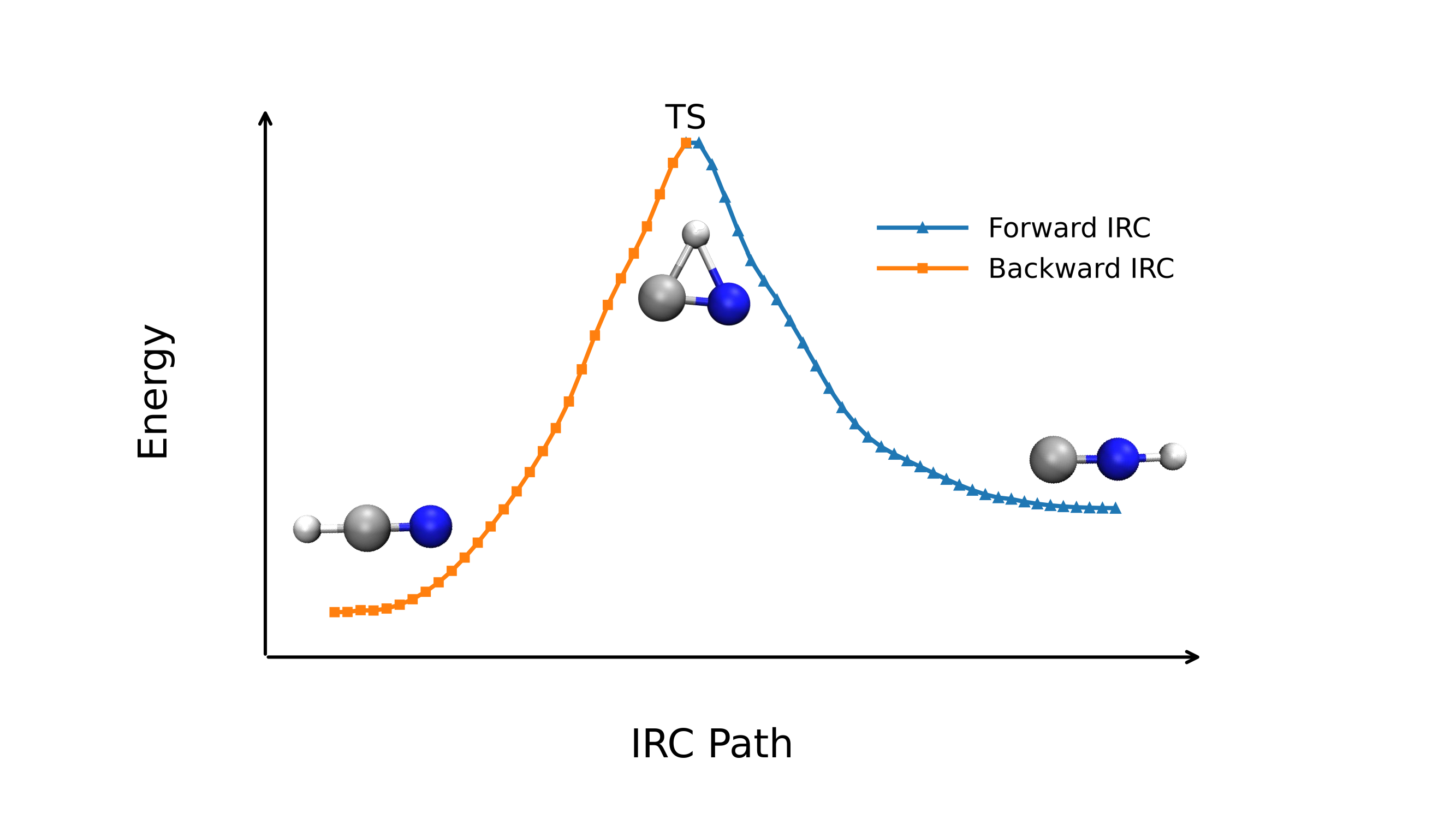
In this example, we will perform the classic isomerization calculation case of the HCN -> HNC. The TS structure is derived via the PRFO method. To speed up the calculation, a larger step size of 0.15 was used.

Input Example

#model=aimnet2nse
#irc(method=lqa,step_length_bohr=0.15)
#device=gpu0

XYZ  0  1  /path/to/transition_state.xyz

Output Visualization

After a brief wait for the calculation to complete, we can visualize the reaction path and the energy profile along the reaction coordinate.

LQA IRC animation — **Trajectory:** Simplified view of the reaction path

LQA IRC graph — **Graph:** Energy trend along the IRC path

Ref Structure

Transition State

3
Iteration 6  Energy = -93.3911999898
C   0.4147189982  0.0090611094 -0.5547979606
N   0.0319422836 -0.0048546467  0.5850722629
H   1.3836904902 -0.1619564366  0.2436923366

Comparison with GS

The LQA and GS methods differ primarily in how they determine each IRC step:

GS uses a pivot-step followed by constrained optimization on a hypersphere. It does not rely on the quadratic approximation for the step direction, making it more robust on surfaces where the quadratic model breaks down.
LQA uses the full quadratic model (gradient + Hessian) to analytically predict the next point, which can be faster when the quadratic approximation is accurate.

In practice, LQA tends to be faster on smooth, harmonic-like surfaces, while GS is more robust for highly anharmonic or strongly curved reaction paths. If LQA has convergence difficulties, switching to GS or HPC is recommended.