Solvation
The #solv(...) command adds solvent treatment before the requested MAPLE task. Current MAPLE exposes two separate modes: an experimental implicit GB-polar/QEq energy correction, or a coordinate-building explicit solvent cluster. Choose one mode per input; implicit and explicit solvent options are intentionally mutually exclusive.
Current scope
Implicit solvation is experimental, energy-only, and currently valid only for #sp. Explicit solvent creates a non-periodic coordinate-only cluster around one input structure; it does not create a periodic box, cell metadata, or automatic frozen outer-shell constraints.
Overview
| Mode | Use | Required syntax | Task support |
|---|---|---|---|
| Implicit GB-polar/QEq | Single-point energy correction from geometry-dependent QEq charges and a heuristic GB-polar model | #solv(method=gbsa, implicit=water, experimental=true) |
#sp only |
| Explicit solvent cluster | Build solvent coordinates from a pure-solvent PDB template around the solute | #solv(explicit=water) |
Pre-processing step before the selected task |
Do not combine implicit=<solvent> and explicit=<solvent> in the same #solv line. Explicit-solvent geometry options such as radius, shape, density, number, solvent_pdb, and clash settings are rejected for implicit jobs.
Implicit GB-polar/QEq
Implicit solvation uses method=gbsa with an implicit solvent name. MAPLE computes QEq charges for the current geometry and adds an experimental GB-polar energy term. Because the QEq charges are geometry-dependent and not variationally coupled to the solvent expression, solvent forces, Hessians, stress, and HVPs are disabled.
#model = uma
#solv(method=gbsa, implicit=water, experimental=true)
#sp
The experimental=true flag is required so the input states that this is an energy-only experimental correction. Use it for single-point energy comparisons, not optimization, MD, transition-state searches, scans that require solvent forces, or frequency calculations.
Implicit solvent names
- acetone
- acetonitrile
- benzene
- cs2
- dichloromethane
- dmf
- dmso
- ether
- methanol
- nhexan
- thf
- toluene
- trichloromethane
- water
Explicit solvent clusters
Explicit solvation reads a pure-solvent PDB template, tiles it in space, crops whole solvent molecules to the requested cluster geometry, removes solute-solvent and solvent-solvent clashes, and appends the accepted solvent coordinates to the solute. The resulting ASE atoms are marked as a non-periodic coordinate-only cluster with pbc=False and a zero cell; MAPLE also writes solvated XYZ/PDB sidecars without a periodic cell record.
#model = uma
#solv(explicit=water, radius=12.0)
#opt(method=lbfgs)
Explicit solvation currently supports exactly one input structure. Remove #pbc for explicit-solvent jobs. If you need to hold solute atoms or selected solvent atoms fixed during an optimization, use the normal constraint commands after the coordinate block; the solvent builder itself only generates coordinates.
For documentation previews, use the generated *_solvated.xyz sidecars directly. The figures below come from the source examples in examples/opt/exp-solv/ before any optimization frames are used.
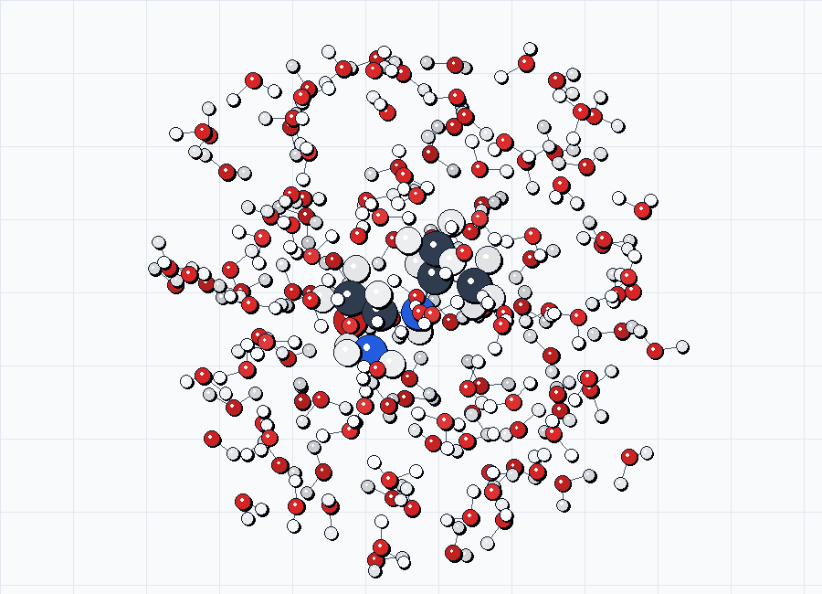
solv1_solvated.xyz.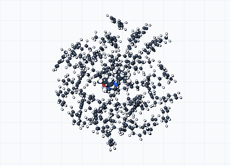
solv2_solvated.xyz.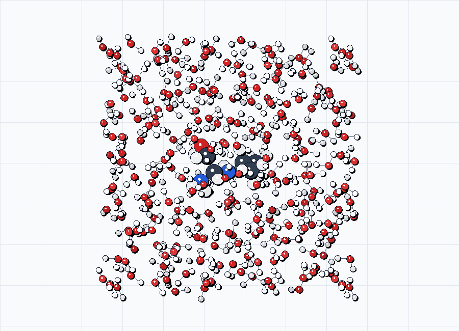
shape=cube, box_size=20.0, default water density.Bundled explicit-solvent templates
The current MAPLE source ships the following explicit-solvent PDB template stems. Use exactly the filename stem as the explicit= value:
2methyl2propanol2methylpyridine4methyl2pentanoneaceticacidacetoneacetonitrileacetophenoneanilineanisolebenzenebenzonitrilebenzylalcoholbromobenzenebromoethanebromoformbromooctanebutanolbutanonebutylacetatebutylbenzenecarbontetchlorobenzenechloroformchlorohexanecyclohexanecyclohexanonedecalindecanedecanoldibromoethanedibutyletherdichloroethanediethylaminediisopropyletherdimethylacetamidedimethylformamidedimethylpyridinedimethylsulfoxidedodecaneethanoletherethoxybenzeneethylacetateethylbenzenefluorobenzenefluoroctaneheptaneheptanolhexadecanehexadecyliodidehexanehexanoliodobenzeneisobutanolisooctaneisopropanolisopropylbenzeneisopropyltoluenemcresolmesitylenemethanolmethoxyethanolmethylenechloridemethylformamidenitrobenzenenitroethanenitromethanenonanenonanoloctaneoctanolodichlorobenzeneold_aceticacidold_tributylphosphateonitrotoluenepentadecanepentanepentanolperfluorobenzenephenyletherpropanolpyridinesecbutanolsecbutylbenzenetbutylbenzenetetrachloroethenetetrahydrofurantetrahydrothiophenedioxidetetralintoluenetributylphosphatetriethylaminetrimethylbenzeneundecanewaterxylene
Two legacy duplicate template stems, old_aceticacid and old_tributylphosphate, are bundled files too; prefer aceticacid and tributylphosphate for new inputs.
Templates with default density values
MAPLE has built-in density values for these explicit-solvent names when neither density= nor number= is supplied:
aceticacidacetoneacetonitrileanilinebenzenebutanolcarbontetchloroformcyclohexanedichloroethanedimethylacetamidedimethylformamidedimethylsulfoxideethanoletherethylacetateheptanehexaneisopropanolmethanolmethylenechloridenitrobenzenenitromethaneoctanepropanolpyridinetetrahydrofurantoluenewaterxylene
For bundled templates, use the template filename stem as the explicit= value. For example, the bundled water.pdb template is selected with explicit=water. If a solvent has no tabulated density, provide density=<g/mL> or number=<int>.
Custom solvent PDB templates
Use solvent_pdb=path/to/template.pdb to provide a custom solvent template. In this mode, solvent_pdb selects the actual PDB file, while explicit=<name> declares the solvent identity represented by that file. MAPLE does not infer the solvent name from the custom PDB filename. Relative solvent_pdb paths are resolved from the input file directory.
For example, the following input reads boxes/water_bulk.pdb because that is the solvent_pdb path. The explicit=water part means “treat this template as water” for the default density lookup, output labels, and water-specific template checks; it is not derived from the filename water_bulk.pdb.
#model = uma
#solv(explicit=water, solvent_pdb=boxes/water_bulk.pdb, density=0.997, radius=14.0)
#opt(method=lbfgs)
A custom template must be a pure-solvent bulk PDB, group one connected solvent molecule per residue, use the same molecular formula for every residue, and contain an orthorhombic CRYST1 record. For explicit=water, each residue must be one H2O molecule. MAPLE unwraps molecules that cross an orthorhombic box boundary before validating connectivity, so GROMACS/OpenMM-style water boxes are acceptable when residue grouping remains correct. If the density implied by CRYST1 does not match MAPLE's default density for the declared explicit=<name>, MAPLE refuses to infer the target density; add an explicit density= matching the template, or use number= to bypass density inference and request an explicit molecule-count target.
Parameters
Mode selection
| Parameter | Mode | Meaning |
|---|---|---|
method=gbsa |
Implicit | Required when using implicit=<solvent> |
implicit=<solvent> |
Implicit | Solvent name for the experimental GB-polar/QEq energy correction |
experimental=true |
Implicit | Required acknowledgement that implicit solvation is experimental and energy-only |
explicit=<solvent> |
Explicit | Bundled solvent template name, or density label when used with solvent_pdb |
solvent=<name> |
Compatibility alias | Interpreted as implicit when method=gbsa is present, otherwise as explicit; prefer implicit= or explicit= |
Explicit cluster geometry and density
| Parameter | Default | Description |
|---|---|---|
shape |
sphere |
sphere crops by molecular-center radius; cube crops by molecular-center box extent |
radius |
10.0 |
Sphere radius in Angstroms; valid only with shape=sphere |
box_size |
required for cube | Cube side length in Angstroms; valid only with shape=cube |
density |
tabulated if available | Mass density in g/mL used to compute the target solvent molecule count |
density_scale |
1.0 |
Multiplier applied to the density-derived target count |
number |
unset | Explicit target solvent molecule count; overrides density-based targeting |
solvent_pdb |
bundled template | Path to a homogeneous pure-solvent bulk PDB template; relative paths are resolved from the input file directory |
Explicit clash handling and output controls
| Parameter | Default | Description |
|---|---|---|
clash_method |
vdw |
vdw removes atoms closer than scaled van der Waals radii; distance uses a fixed distance tolerance |
vdw_scale |
0.57 |
Scale factor for vdW clash thresholds when clash_method=vdw |
vdw_fallback_radius |
1.05 |
Fallback vdW radius in Angstroms for elements without a tabulated radius |
tolerance |
2.0 |
Fixed-distance clash cutoff in Angstroms when clash_method=distance |
clash_cutoff |
alias for tolerance |
Compatibility name that selects clash_method=distance |
randomize |
true |
Randomize template phase and rigid rotation before tiling |
seed |
0 |
Reproducible random seed; use seed=-1 for non-reproducible sampling |
write_shell |
false |
Write additional solute-centered shell sidecars when set to true |
shell_cutoff |
required with write_shell=true |
Keep whole solvent molecules whose closest atom is within this distance of the solute in the shell output |
Examples
Energy-only implicit water single point
#model = uma
#device = gpu0
#solv(method=gbsa, implicit=water, experimental=true)
#sp

0 1
C    0.000000    0.000000    0.000000
C    1.501000    0.000000    0.000000
O    2.098000    1.060000    0.000000
H   -0.392000    1.011000    0.000000
H   -0.392000   -0.506000    0.875000
H   -0.392000   -0.506000   -0.875000
H    1.960000   -1.003000    0.000000
Explicit water cluster for optimization
#model = uma
#device = gpu0
#solv(explicit=water, radius=10.0, seed=0)
#opt(method=lbfgs, level=medium)

0 1
C    0.000000    0.000000    0.000000
C    1.501000    0.000000    0.000000
O    2.098000    1.060000    0.000000
H   -0.392000    1.011000    0.000000
H   -0.392000   -0.506000    0.875000
H   -0.392000   -0.506000   -0.875000
H    1.960000   -1.003000    0.000000
Cube-shaped explicit cluster with a target count
#model = uma
#solv(explicit=water, shape=cube, box_size=20.0, number=120, clash_method=vdw)
#sp

XYZ /path/to/solute.xyz
Write a smaller analysis shell sidecar
#model = uma
#solv(explicit=water, radius=14.0, write_shell=true, shell_cutoff=5.0)
#sp

XYZ /path/to/solute.xyz
The main solvated coordinate sidecars contain the generated full cluster. With write_shell=true, MAPLE also writes smaller _cluster.xyz and _cluster.pdb files containing the solute plus whole solvent molecules within shell_cutoff.
Limitations and best practices
- Pick one solvent mode: use implicit GB-polar/QEq or explicit solvent coordinates, not both in one job.
- Treat implicit as energy-only: run it with
#spandexperimental=true; do not use it for jobs that need solvent forces or Hessians. - Keep explicit clusters non-periodic: remove
#pbc; MAPLE does not write cell metadata for explicit clusters. - Control density deliberately: use the default density table for common solvents, or specify
density=/number=for custom templates and unusual solvent names. - Prefer vdW clash filtering: the default
clash_method=vdwis usually safer than a single fixed distance across all elements; useclash_method=distanceonly when you intentionally want a fixed cutoff. - Validate custom templates: the template should be homogeneous pure solvent, have one connected molecule per residue, and include an orthorhombic
CRYST1box consistent with the density you request or the explicitnumber=target. - Expect finite clusters: small unconstrained solvent clusters may move during optimization. Increase the radius/count, write an analysis shell, or add ordinary MAPLE constraints when a specific region must remain fixed.